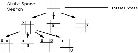
State space Search

3.1.3 - State space representation of problem

Example: Representing Xs and Os as state-space problem.
Image courtesy of Ralph Morelli.
See Luger Fig II.5

State space representation of a problem:

All the states the system can be in are represented as nodes of a graph.
An action that can change the system from one state to another (e.g. a move in a game) is represented by a link from one node to another.
Links may be unidirectional (e.g. Xs and Os, can't go back) or bi-directional (e.g. geographic move).
Search for a solution.
A solution might be:
1. Any path from start state to goal state.
2. The best (e.g. lowest cost) path from start state to goal state (e.g. Travelling salesman problem).
It may be possible to reach the same state through many different paths (obviously true in Xs and Os).
There may be loops in the graph (can go round in circle). No loops in Xs and Os.

Xs and Os

Xs and Os
Directed acyclic graph
Unidirectional. No loops. Multiple paths to the same state.
Multiple goal states.
Game-tree complexity
- 9 first moves, 8 replies, 7 replies, ...
- 9! (9 factorial) = 362,880 different paths.
- In fact, 9! is an upper bound - many of these games will terminate with a win before reaching end of path.
- Number of paths < 9!
- Unlike chess, could do exhaustive search.
State-space complexity
- How many unique states exist?
- Could have blank, X or O in each of 9 squares.
- That is 3⁹ = 19,683 different states.
- In fact, this is an upper bound - many of these states don't exist. e.g. 9 X's.
- These states don't exist:
  1. (Number of Xs) - (Number of Os) = 2 or more
  2. (Number of Os) - (Number of Xs) = 2 or more
- Q. Is this a complete list of non-existent states?

Reduce statespace

We can use symmetry reduction to reduce the search problem.
Many states are rotations or mirror-image of another state, so we don't have to search them separately.
e.g. There are basically only 3 unique first moves.

See Luger Fig 4.1

Symmetry reduction on 1st level reduces no. of paths to 3 . 8!
Symmetry reduction on 2nd level reduces no. of paths to 12 . 7! = 60,480

Symmetry reduction may require a lot of work by the human. But worth it if it reduces search problem (sometimes massively).
We write code to do the transform, search and transform back.

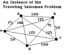
Travelling salesman problem (TSP)

Travelling salesman problem

Travelling salesman problem.
Start at A, visit all cities, return to A. Links show cost of each trip (distance, money). Find trip with minimum cost.
Solution is a path. e.g. [A,D,C,B,E,A]
Image courtesy of Ralph Morelli.
See Luger Fig 3.9

Q. What is the shortest path?

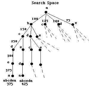
Representing Travelling salesman problem as state-space problem.
Image courtesy of Ralph Morelli.
See Luger Fig 3.10.
Start at A, 4 choices for first step, 3 choices for next, 2 choices, 1 choice.
4! (4 factorial) paths = 24 paths

Q. What assumption did we make?

Q. When do we stop the search?

How big is the TSP?

In general, how many paths are there in the TSP?

Given n cities, (n-1) choices for 1st stop, (n-2) choices for next stop, etc.
Q. What assumption did we make?
(n-1)! paths
With many cities or nodes this soon becomes intractable.

Restrict search / Problem-specific heuristics

With problems that scale badly, we need to restrict the search in some way.
Many of these restriction ideas will be problem-specific - the idea only works on this problem and not on all problems.

Reduce statespace

Branch and bound
- Keep track of best path so far. This is a bound on future candidates.
As soon as best possible extension to a partially-constructed path (the branch) exceeds bound, that partial path and all its extensions are removed.
Reduces space but still exponential (const)ⁿ number of paths.

Heuristic search

With large state spaces (e.g. 50 cities) need to use heuristic.
e.g. Nearest neighbour: "Go to the nearest unvisited city."
Finds solution quick! (Only tries one path!)

Luger changes his numbers to show example of "Nearest neighbour" heuristic failing on Travelling salesman problem:

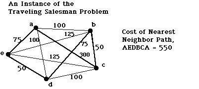
Image courtesy of Ralph Morelli.
See Luger Fig 3.11

3.2 - Searching a statespace graph

3.2.2 - Backtracking (exhaustive search)

Backtracking - exhaustive search, try each path in order, until find goal.

Depth-first search

The "Depth-first search" version of exhaustive search.
Goes down to remote descendants looking for solution before back-tracks up to a sibling.

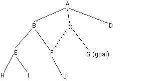
Depth-first search:
Start at A. Search state space systematically until find goal.
When multiple children, go down 1st child. If fails, back to parent, down 2nd child, and so on.
Image courtesy of Ralph Morelli.
See Luger Fig 3.14

Note there are multiple paths to F.
If F has already been found to be a dead-end when we went there from B, the algorithm should not go there a second time (from C).
However not a great example here since C can see goal so won't go to F anyway.

Breadth-first search

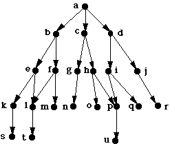
The "Breadth-first search" version of exhaustive search.
Search all children (siblings) before search all grandchildren.

Image courtesy of Ralph Morelli.

Depth-first search examines the nodes in the order:

  A, B, E, K, S, L, T, F, M, C, G, N, H, O, P, U, D, I, Q, J, R

Need to:

Keep track of current path from start. Keeps changing as we search down.
Keep track of dead ends - have searched all below this state.
Keep track of known states not yet searched - will be quite small.

Breadth-first search does each level first before moving lower, examines the nodes in the order:

  A, B, C, D, E, F, G, H, I, J, K, L, M, N, O, P, Q, R, S, T, U

Need to:

Keep track of known states not yet searched - will grow massively, since it is all cousins at the current level down.