Research - PhD - Acknowledgements - Appendix A

A Incremental sampling of random variables

Most of the results in these appendices are either well-known or trivial, but they are included here for completeness, and so they can be referred to from the main body of the text.

A.1 Single variable (average)

Let

be samples of a stationary random variable d with expected value E(d). Then the following update algorithm provides an elegant way of sampling them. Repeat:

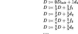
Proof: D's updates go:

displaymath9187

i.e. D is simply the average of all samples so far.

As , .

More generally:

Proof: D's updates go:

displaymath9188

As :

that is, .

One way of looking at this is to consider as the average of all samples before time t, samples which are now irrelevant for some reason. We can consider them as samples from a different distribution f:

Hence:

displaymath9191

as .

I could have made this clearer:
1/n ( d_t + ... + d_n ) = (n-t+1)/n 1/(n-t+1) ( d_t + ... + d_n )
-> 1 . E(d)

A.2 Single variable (time-weighted)

An alternative approach (e.g. see [Grefenstette, 1992]) is to build up not the average of all samples, but a time-weighted sum of them, giving more weight to the most recent ones. This is accomplished by setting to be constant, in which case D's updates go:

displaymath9240

Since as , this weights more recent samples higher. Grefenstette uses typically .

A.3 Multiple variables

Consider sampling alternately from two stationary random variables d and f:

displaymath9250

Proof: From Theorem A.1, after 2t samples:

displaymath9251

as .

More generally, consider where we have multiple stationary distributions , where each distribution has expected value . At each time t, we take a sample from one of the distributions. Each distribution has probability p(i) of being picked. Repeat:

Proof: For a large number of samples t we expect to take p(1) t samples from , p(2) t samples from , and so on. From Theorem A.1, we expect:

displaymath9253

as .

Appendix B

Return to Contents page.