Chaos Theory demo

The Logistic map

This demonstrates the chaotic process that may result when you repeatedly apply the update:

x := λ x (1-x)

for certain values of λ (lambda) and certain starting values of x in the range:

0 < x < 1

(Note that starting with x=0 or x=1 will just cause x:=0 forever.)

I often use := for assignment to distinguish from = for equality.

List of chaotic maps
- Logistic map (and here)
The Logistic Map and Chaos
Vivaldi, Franco (1992), "An experiment with mathematics", The New Scientist guide to Chaos.

Initial notes

First note that the maximum value of x * (1-x) is at x = 0.5 (see proof).
At x = 0.5, the product equals 0.25. So for the equation to again yield a value between 0 and 1, we want:

0 < λ < 4

(λ=0 obviously causes x:=0 forever.)

0 < λ < = 1

Note that x * (1-x) is strictly less than x, so if λ is less than or equal to 1, the series goes eventually to zero. e.g. λ=0.5, x=0.5.

1 < λ < = 3

If λ is greater than 1, there is a stable solution at:
x = 1 - (1/λ)
= (λ-1) / λ

For example, put λ = 2. You will see that the stable solution for the equation is x = 0.5. You will also see that for any starting value of x from 0 to 1, the process will actually converge to this stable value x = 0.5, e.g. try starting at 0.1 or 0.9.

It is known (though not proved here) that for 1 < λ < = 3 the process will converge to the stable solution. Though for precisely 3, convergence is dramatically slow.

At λ = 2.5, stable solution = 0.6, start also at 0.61 or 0.1 or 0.9.

At λ = 2.9, stable solution = 19/29 = 0.65517241379310344827586206896552, but convergence time is increasing, start at 0.655 or 0.6.

At λ = 3, stable solution = 2/3 = 0.6666666666666666666666666666666667, but convergence time very long, start at 0.666 or 0.6 or 0.1.

3 < λ < 3.569945672

Next, try λ = 1 + √5 = 3.2360679775. The stable solution is √5 / (1 + √5) = 0.6909830056251. However, you will notice very strange behaviour. Unless you start at exactly the stable value, it will rapidly diverge from the stable solution and end up bouncing between 2 "attractor" values, 0.5 and (1 + √5) / 4 = 0.8090169943749, forever, e.g. try starting at 0.69.

Q. For λ = 1 + √5, is one of the attractors exactly 0.5?
Prove it either way (by applying update twice and seeing if get back to 0.5 exactly).

Now try λ = 3.5. Again, there is a stable solution (at x = 5/7 = 0.7142857142857), but again it is largely irrelevant because all other values end up in an attractor cycle. Note that as we increase λ, the length of the cycle is increasing. Now the cycle is of length 4, e.g. start at x = 0.875.

Q. For λ = 3.5, is one of the attractors exactly 0.875?
Prove it either way (by applying update 4 times and seeing if get back to 0.875 exactly).

The length of the cycle goes to infinity as λ increases.

In fact, the length of the cycle goes to infinity as λ goes to a constant (the "accumulation point") which is approximately 3.569945672. Between approximately 3.569945672 and 4, we have new behaviour.

3.569945672 < = λ < = 4

In this region, the map seems to generate an infinite sequence of unrelated random numbers between 0 and 1.

Oddly enough, there are sub-regions in which oscillation between a few values occurs again.
e.g. λ = 1 + √8 = 3.82842712474619009760
Stable soln 0.73879612503625855748588356095603.
Other start values bounce between 3 values.
Start at 0.16.

From now, we will look at λ = 4, for which there are no oscillations.

λ = 4

A finite number of real numbers will lead to 0 convergence in finite steps

With λ = 4, anything that leads to 0.5 will lead to 0 forever. e.g. Starting at 0.5. But also starting at either of the 2 numbers where λ * x * (1-x) = 0.5. Namely (1+(1/√2))/2 = 0.853553391 and (1-(1/√2))/2 = 0.146446609. Or starting at any of the 4 numbers that lead to one of these 2. And any of the 8 numbers that lead to those. And so on. These go to 0 eventually, but the time taken to go to 0 is increasing.

In general, given any number c between 0 and 1, there are exactly 2 solutions, both between 0 and 1, to:

4 x (1-x) = c

We can see this as follows:
4x - 4x² = c
4x² - 4x + c = 0
(Quadratic Equation)
x = ( 4 ± √(16 - 16c) ) / 8
= ( 1 ± √(1-c) ) / 2

Now c is between 0 and 1, so (1-c) is, so √1-c is.
So (1 + √1-c) / 2 is between 1/2 and 1.
And (1 - √1-c) / 2 is between 0 and 1/2.
Each solution is of course (1 - the other solution).
So we have 2 unique numbers that lead to c after 1 more iteration.

x = 0.5     - goes to 0 after 2 steps
2 numbers   - go to 0 after 3 steps
4 numbers   - go to 0 after 4 steps
2^3 numbers - go to 0 after 5 steps
2^4 numbers - go to 0 after 6 steps
...

If we consider a sequence of any finite length n, there are a finite number of 2^(n-2) real numbers in the interval 0 to 1 that have converged to 0 at the end of that sequence of n iterations. Obviously, there are an infinite number of real numbers that have not.

Stable solution 0.75

You can see that again there is a stable solution at x = 0.75.

A finite number of real numbers lead to 0.75 convergence in finite steps

Similar to above, we consider the numbers that lead to 0.75:

x = 0.75    - goes to 0.75 after 0 steps
2 numbers   - go to 0.75 after 1 steps
4 numbers   - go to 0.75 after 2 steps
2^3 numbers - go to 0.75 after 3 steps
2^4 numbers - go to 0.75 after 4 steps
...

If we consider a sequence of any finite length n, there are a finite number of 2ⁿ real numbers in the interval 0 to 1 that have converged to 0.75 at the end of that sequence of n iterations. Obviously, there are an infinite number of real numbers that have not.

There are an infinite number of other real numbers

Apart from the finite number of real numbers that converge to 0 or 0.75 in any finite time, there are an infinite number of other real numbers.

If the starting value of x is 0.75 it will stay at that value forever. However, other starting values (apart from the unusual special cases just listed) do not converge to 0.75, or indeed to anything, e.g. try starting at x = 0.7. You will see that values bounce around randomly in the interval between 0 and 1 forever. The length of the attractor cycle has gone to infinity. Even try starting at x = 0.7501. You will see that it will rapidly diverge from 0.75, and never go back.

This illustrates the classic chaotic property that tiny initial differences lead to massive differences later. Here is a system that is deterministic yet unpredictable.

The function f

Define the function f as follows:

Let f(x) = the result of applying the update to x 29 times with λ = 4.

i.e. f(x) = the last line of the sequence here. There are 2²⁷ real numbers for which f(x)=0 converged. There are 2²⁹ real numbers for which f(x)=0.75 converged. And there are an infinite number of other real numbers whose f values go all over the interval 0 to 1. Note that it is symmetric: f(c) = f(1-c).

What does f look like?

Imagine drawing f(x). Plot f(x) for x = 0.75001, 0.75002, 0.75003, 0.75004, ... Hard to draw isn't it? f(x) bounces all over between 0 and 1. Tiny change in x leads to massive change in f(x). Consider:

f(0.751) = 0.16135
f(0.752) = 0.62721
f(0.753) = 0.04611
f(0.754) = 0.81176

A smooth curve going up between 0.751 and 0.752?
No. It bounces around in that interval:

f(0.751) = 0.16135

f(0.7511) = 0.96567
f(0.7512) = 0.74842
f(0.7513) = 0.97527
f(0.7514) = 0.08098
f(0.7515) = 0.63691
f(0.7516) = 0.23017
f(0.7517) = 0.68586
f(0.7518) = 0.12163
f(0.7519) = 0.49033

f(0.752) = 0.62721

A smooth curve going up between 0.751 and 0.7511?
No. It bounces around in that interval:

f(0.751) = 0.16135

f(0.75101) = 0.32690
f(0.75102) = 0.43537
f(0.75103) = 0.46383
f(0.75104) = 0.40957
f(0.75105) = 0.27892
f(0.75106) = 0.10807
f(0.75107) = 0.00091
f(0.75108) = 0.12277
f(0.75109) = 0.54406

f(0.7511) = 0.96567

and so on, for all the other tiny intervals.

Plotting f

Here we plot in steps of 0.1 with gnuplot:

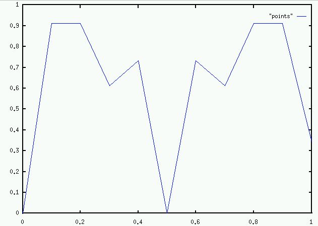
Note it is symmetric: f(c) = f(1-c).
f(0) = 0. f(0.5) = 0. f(1) should be = 0 but is not because of a compiler bug.

Is this what f looks like? No. Let's plot in steps of 0.01:

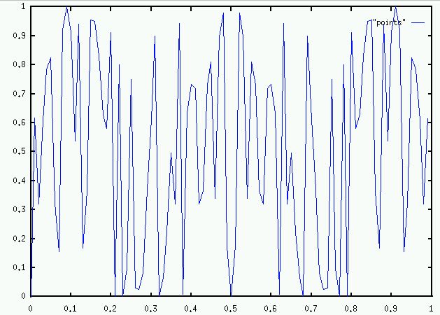
Is this what f looks like? No. Let's plot in steps of 0.001:

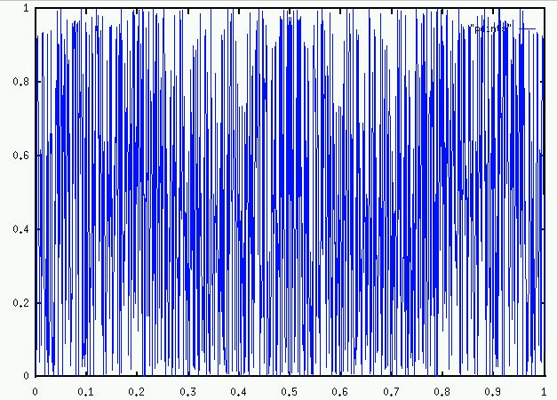
Is this what f looks like? No. Let's plot in steps of 0.0001:

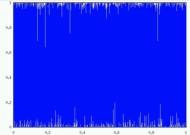
gnuplot can't really draw it. To draw it is to more or less just fill the square (x=0 to x=1, y=0 to y=1) with points.

Q. Is it really to fill the square with points?

Close-up

Maybe with more magnification we can see it is a function?
We try a close-up of the area between 0 and 0.01.

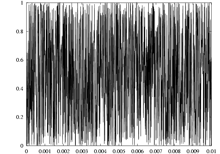
This does 1000 samples between 0 and 0.01.
Is that all the detail there is? No:

This does 10,000 samples between 0 and 0.01.

λ > 4

Try λ just slightly greater than 4. You may be surprised at what happens. e.g. λ=4.1, x=0.001.

Q. Does it always go to minus infinity?