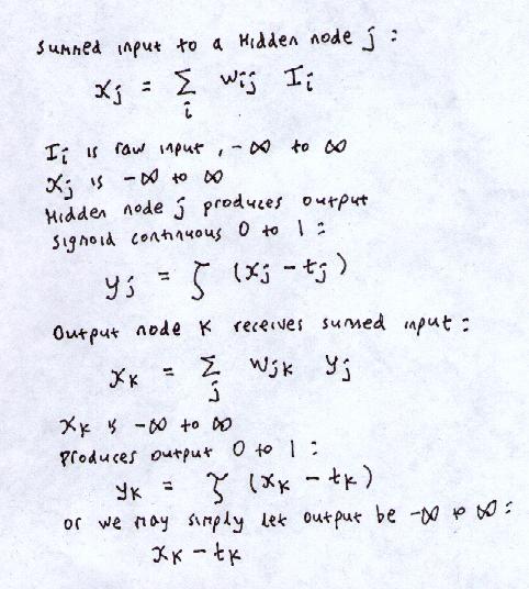
The "Back-propagation" learning algorithm

We will now define a learning algorithm for Multi-layer Neural Networks.

We assume the network will use the Sigmoid activation function.

Notation

Note: Not a great drawing. Can actually have multiple output nodes.

Input can be a vector.
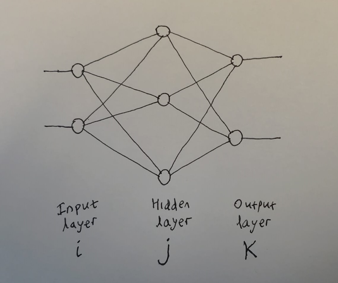
There may be any number of hidden nodes.
Output can be a vector too.

Typically fully-connected. But remember that if a weight becomes zero, then that connection may as well not exist. Learning algorithm may learn to set one of the connection weights to zero. i.e. We start fully-connected, and learning algorithm learns to drop some connections.

To be precise, by making some of its input weights w_ij zero or near-zero, the hidden node decides to specialise only on certain inputs. The hidden node is then said to "represent" these set of inputs.

Remove thresholds

First, we are going to get rid of the thresholds. (This will be explained later.)

So we have:

and:

Error term

We sent in an input, and it generated, in the output nodes, a vector of outputs y_k.
The correct answer is the vector of numbers O_k.
The error term is:

We take the squares of errors, otherwise positive and negative errors may cancel each other out.

Q. Show example of where error term fails if we don't take the squares.

There are other possible measures of error (recall Distance in n-dimensions) but we can agree that if this measure -> 0 then all other measures of error -> 0

Q. Prove that if this measure of E = 0 then y_k = O_k for all k.

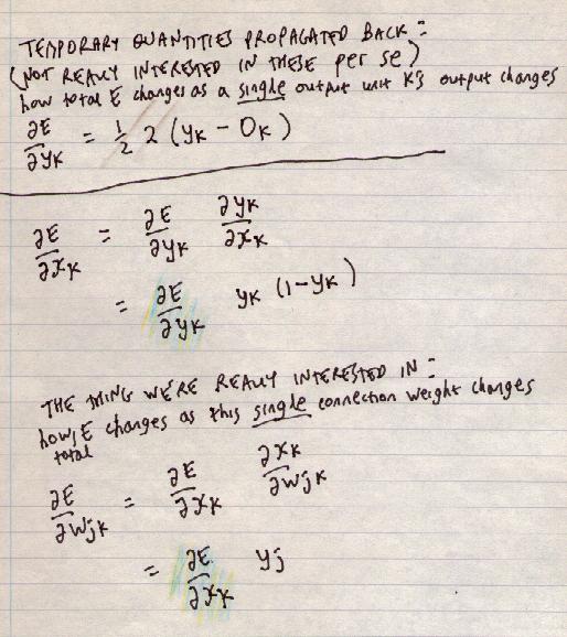
The Learning algorithm - Back-propagation

To look at how to reduce the error, we look at how the error changes as we change the weights. We start at the layer immediately before the output. Working out the effects of earlier layers will be more complex.

First we can write total error as a sum of the errors at each node k:

E = Σ _k E_k

where E_k = 1/2 (y_k - O_k)²

Now note that y_k, x_k and w_jk each only affect the error at one particular output node k (they only affect E_k).
So from the point of view of these 3 variables, total error:

E = (a constant) + (error at node k)

hence:

(derivative of total error E with respect to any of these 3 variables) = 0 + (derivative of error at node k)

e.g.

∂E/∂y_k = 0 + ∂E_k/∂y_k

We can see how the error changes as y_k changes, or as x_k changes. But note we can't change y_k or x_k - at least not directly. They follow in a predetermined way from the previous inputs and weights.

But we can change w_jk

partial derivatives

E is a function of many variables.
We will be repeatedly holding all except one constant and seeing how E changes as just one variable is changed.
This is what we mean by using partial derivatives (also here).

Derivatives of E - output layer:

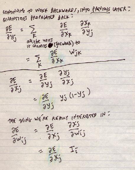
As we work backwards, the situation changes. y_j feeds forward into all of the output nodes. Since:

E = (sum of errors at k)

we get:

(derivative of E) = (sum of derivatives of error at k)

x_j and w_ij then only affect y_j (though y_j affects many things).

We can't (directly) change y_j or x_j

But we can change w_ij

Derivatives of E - previous layer:

To spell it out:
∂E/∂y_j = Σ _k ∂E_k/∂y_j
= Σ _k ∂E_k/∂x_k ∂x_k/∂y_j
= Σ _k ∂E/∂x_k ∂x_k/∂y_j

Error landscape: Changing the weights to reduce the error

Now we have an equation for each - how error changes as you change the weight.

Note some things:

E >= 0 - it can't be negative.
So we can't have the line just going down forever. It must level out. Get slope = 0 at some point (perhaps many points).
In fact, might not be able to get E = 0 for all exemplars given limited net architecture, so best E might still be > 0.
W can be negative. In fact, best W might be.
As W -> infinity (or minus infinity) error almost certainly gets very bad. Best W will be something finite.

Now, to reduce error:

On RHS, slope is positive: > 0.
Move left to reduce error:
W := W - C
where C is a positive constant.
On LHS, slope is negative: < 0.
Move right to reduce error:
W := W - C
= W - C (negative quantity)
= W + (positive quantity)

Hence the same update rule works for both positive and negative slopes:

W := W - C

The constant C is the LEARNING RATE
C > 0
Typically C < 1
(In the code we can try a wide range of C and see what happens.)

That's how we learn the weights. How do we learn thresholds?

Remember definition of threshold if using sigmoid function.
sigmoid(x-t) instead of sigmoid(x)

Biasing: Just make the thresholds into weights, on a link with constant input -1.

So instead of:

we change it to:

and we just learn the thresholds like any other weights.

i.e. Every single hidden unit (and every single output unit) has an extra input line coming apparently from nowhere with constant input -1.

We need thresholds

Remember we need thresholds, otherwise the sigmoid function is centred on zero. e.g. If no thresholds, then, no matter what the exemplars are, no matter what the I/O relationship is, and no matter what the weights are, if all inputs are 0, then output of every single hidden node is ..

Q. Is what?

Similarly, for a node that specialises on n of the inputs (weight = 0 for others), then if that subset of inputs are all 0, that node's output must be ..

Summary: The Back-propagation algorithm

We can now put everything together. The algorithm is:

Repeat:

Send in inputs I_i for this exemplar.
Calculate outputs y_k
Get given correct outputs O_k
Measure E.
w_jk weights:
1. Calculate all the = y_k ( 1 - y_k ) ( y_k - O_k )
2. Calculate all the = y_j
3. For all j,k:
w_ij weights:
1. Calculate all the = y_j ( 1 - y_j ) Σ _k ( w_jk )
2. Calculate all the = I_i
3. For all i,j:
Repeat (next exemplar).

See C++ sample code.
Compare with Perceptron Learning Rule.

Summary of how it responds to errors

Note that y_j is positive, and y_k(1-y_k) is positive, so if (y_k-O_k) is positive (i.e. output is too big), then is positive, and our learning rule reduces the weights. This will reduce the output.
Similarly you can see that if the output y_k is too small, the learning rule increases the weights, which will increase the output.
Note that if E = 0, the update rule will cause no change in weights w_ij or weights w_jk. Why?
Note that if I_i = 0, none of the weights w_ij (for all j) will be changed. Why? Why is this a good thing?
Note that if y_j = 0, none of the weights w_jk (for all k) will be changed. Why? Why is this a good thing?