We will test the action selection methods in use in the hypothetical world of a "house robot". The house robot is given a range of multiple parallel and conflicting goals and must partially satisfy them all as best as it can. We will test Q-learning and Hierarchical Q-learning in this world, and then introduce a number of new methods, implementing and testing each one as it is introduced.
Consider what kind of useful systems might have multiple parallel, partially-satisfied, non-terminating goals. Inspired by a familiar such system, the common household dog, I asked the question: What could an autonomous mobile robot do in the home?
Consider that the main fears of any household are (a) fire, (b) burglary and (c) intruders/attackers. These all tend to happen because there is only one or no people at home or the family is asleep. At least, none of these things would happen if there were enough alert adults wandering round all the time.
So in the absence of enough alert adults, how about an alert child's toy? Even if about all a small mobile robot could do was cover ground and look at things, it might still be useful. In this hypothetical scenario, the robot would be a wandering security camera, transmitting pictures of what it saw to some remote mainframe. Imagine it as a furry, big-eyed, child's toy, with no weapons except curiosity. The intruder breaks into the house and the toy slowly wanders up to him and looks at him, and that's it. There's no point in him attacking it since his picture already exists somewhere remote. If the continuous signal from the robot is lost, some human will come and investigate. The house robot could also double as a mobile wandering smoke alarm, and default perhaps to a vacuum cleaner when nothing was happening.
![]() I have collected some
"house robot" links.
I have collected some
"house robot" links.
Microworlds have (very often justifiably) a bad press, so I must state from the outset that I am not interested in realism but in producing a hard action selection problem, and also one that is different from the normal ones encountered say in animal behavior. A more detailed defence of this problem follows shortly.
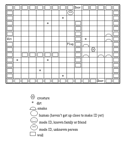
Figure 4.1: The House Robot problem.
Here, the building is on fire, dirt is scattered everywhere,
and a stranger is in the house.
In the artificial grid-world of Figure 4.1,
the positions of entrances
and internal walls are randomised on each run.
Humans are constantly making random crossings from one entrance to another.
The creature (the house robot) should avoid getting in the way of family,
but should follow strangers.
It must go up close first to identify the human as family or stranger.
Dirt trails after all humans.
The creature picks up dirt
and must occasionally return to some base to re-charge and empty its bag.
Fire starts at random and then grows by a random walk.
The creature puts out the fire on a square by moving onto it.
The world is not a torus
- the creature is blocked by inner walls and outer walls
and also can't leave through the
entrances.[1]
The creature can only detect objects in a small radius around it
and can't see through walls
- with the exception of smoke, which can be detected even if a wall is in the way.
Each time step,
the creature senses state ![]() where:
where:
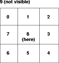
The creature takes actions a, which take values 0-7 (move in that direction) and 8 (stay still).
The fact that its senses are limited, and that there are other, unpredictably behaving entities in the world, means that we must give up on being able to consistently predict the next state of the world. For example, AI planning techniques that assume a static world would be of limited use. The creature must be tightly coupled to the world by continuous observation and reaction.
Given its limited sensory information, the creature needs to develop a reactive strategy to put out fire, clean up dirt, watch strangers, and regularly return to base to re-charge. When we specify precisely what we want, we find that the optimum is not any strict hierarchy of goals. Rather some interleaving of goals is necessary, with different goals partially satisfied on the way to solving other goals. Such goal-interleaving programs are difficult to write and make good candidates for learning.
|
Movie demo of the House Robot problem. |
This artificial world was not constructed to be a simulation of a robot environment. There is no attempt to simulate realistic robot sensors. There is no explicit simulated noise, though we do have limited and confusing sensory information. All I am interested in is setting up a hard action selection problem. And it is hard, as we shall see.
Tyrrell [Tyrrell, 1993, §1.1] defends the value of such microworld experiments in relation to the Action Selection problem at least. At the moment, it is difficult enough to set up a robotics experiments with a single goal. It is still harder to set up multiple conflicting goals and pose decent action selection problems to them.
We can see how far this is from actual robotics. It is unrealistic to think that the robot could reliably classify objects in the world as "dirt", "wall" etc, based on its senses. In fact, it seems to imply that the job of perception is to translate sensory data into symbolic tags. In fact, I make no such claim. I am merely trying to construct a hard action selection problem in a way that we can think about it easily, understand its difficulty, and suggest possible strategies.
Similarly, the actions here (of moving in a particular direction) may actually need to be implemented using lower-level mechanisms. Again, the object is to concentrate on the higher-level problems of the overall strategy.
Since the methods we will test take as input any vector of numbers, and can produce any vector as output, they can be reapplied afterwards to other problems with more realistic sensory and motor data. RL has been applied e.g. by [Mataric, 1994] to multiple, real autonomous mobile robots. I make no stronger assumptions about the world than RL does, so if RL can be applied to real robots then so can my work.
Also this work is not just about robotic or animal-like behavior problems. We are addressing the general issue of a system with multiple conflicting parallel goals. The model could be applied, for example, to such problems as lift scheduling, intelligent building control or Internet agents (see [Charpillet et al., 1996]).
Much time is often spent on the visual user interface of such artificial worlds. But the only important thing is the actual problem to be solved.
In my implementation, I rigorously separate the essential part of the program, the equations to be solved to represent interaction with the world, from the unessential part, any visual representation showing on-screen what is happening. As a result, I can do long learning runs in hidden, overnight batch jobs, being just number-crunching with no user interface at all.
Both the artificial world and the learning algorithms here were implemented in C++.
Note that sensing direction but not distance means that
features of the world that are deterministic
can actually appear probabilistic to the agent.
This is illustrated in Figure 4.3.
When in the situation on the left, the agent will experience:
![]() ,
, ![]() ,
, ![]() .
When in the situation on the right, the agent will experience:
.
When in the situation on the right, the agent will experience:
![]() ,
, ![]() ,
, ![]() .
.
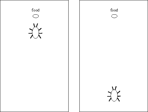
Figure 4.3: Probabilistic transitions ![]() .
.
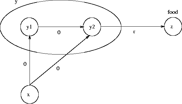
Figure 4.4: Non-stationary probabilistic transitions ![]() .
The states' positions in the diagram correspond to their geographical positions.
x is the state "food is EastNorthEast".
y is the state "food is East".
The agent sees both y1 and y2 as the same state y.
The quantities on the arrows are the rewards for that transition.
.
The states' positions in the diagram correspond to their geographical positions.
x is the state "food is EastNorthEast".
y is the state "food is East".
The agent sees both y1 and y2 as the same state y.
The quantities on the arrows are the rewards for that transition.
In fact, as shown in Figure 4.4, the world is not exactly an MDP.
![]() leads to state y, and
leads to state y, and ![]() also leads to state y.
But the probability of
also leads to state y.
But the probability of ![]() leading to an immediate reward
depends on the agent's policy.
If it tends to take action
leading to an immediate reward
depends on the agent's policy.
If it tends to take action ![]() , the value of y will be higher
than if it tends to take action
, the value of y will be higher
than if it tends to take action ![]() .
But it will not necessarily learn to take action
.
But it will not necessarily learn to take action ![]() as a result
- that would just be normal learning, where it can tell the states apart.
as a result
- that would just be normal learning, where it can tell the states apart.
![]() is just as likely a policy
because
is just as likely a policy
because ![]() is also rewarded when the value of y increases.
is also rewarded when the value of y increases.
![]() is non-stationary.
In fact, the artificial world is a Partially-Observable MDP
[Singh et al., 1994].
But it is very much a non-malicious one,
and can be reasonably approximated as a probabilistic MDP
- this will be proved shortly by the success of RL techniques
when compared against hand-coded solutions in this world.
is non-stationary.
In fact, the artificial world is a Partially-Observable MDP
[Singh et al., 1994].
But it is very much a non-malicious one,
and can be reasonably approximated as a probabilistic MDP
- this will be proved shortly by the success of RL techniques
when compared against hand-coded solutions in this world.
The first method we apply in this world is a single monolithic Q-learning agent learning from rewards.
Reinforcement Learning is attractive because it propagates rewards into behavior, and presumably reward functions (value judgements) are easier to design than behavior itself. Even so, designing the global reward function here is not easy (see [Humphrys, 1996, §4.1] for an example of accidentally designing one in which the optimum solution was to jump in and out of the plug non-stop). Later we will ask if we can avoid having to design this explicitly:
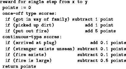
Note that our global reward function, in looking at things from the house's point of view,
actually refers to information that may not be in the state x,
e.g. "fire exists" causes punishment even if the creature cannot see the fire.
From the creature's point of view, this is a stochastic global reward function,
punishing it at random sometimes for no apparent reason.
Such a stochastic reward function is not disallowed under our Markov framework
provided that ![]() is stationary.
is stationary.
The number of possible states x is 1.2 million, and with 9 possible actions we have a state-action space of size 10.8 million. To hold each Q(x,a) explicitly as a floating point number, assuming 4 byte floats, would therefore require 40 M of memory, which on my machine anyway was becoming impractical both in terms of allocating memory and the time taken to traverse it. On many machines, 40 M is not impractical, but we are approaching a limit. Just add two more objects to the world to be sensed and we need 4000 M memory.
In any case, perhaps an even more serious problem is that we have to visit all 10.8 million state-action pairs a few times to build up their values if data from one is not going to be generalized to others. So for reasons of both memory and time, instead of using lookup tables we need to use some sort of generalisation - here, multi-layer neural networks.[2]
Following Lin [Lin, 1992],
because we have a small finite number of actions
we can reduce interference by breaking the state-action space up
into one network per action a.
We have 9 separate nets acting as function approximators.
Each takes a vector input x and
produces a floating point output ![]() .
Each net is responsible for a different action a.
This also allows us to easily calculate the
.
Each net is responsible for a different action a.
This also allows us to easily calculate the ![]() term
- just enumerate the actions and get a value from
each network.[3]
term
- just enumerate the actions and get a value from
each network.[3]
We also note that, as in [Rummery and Niranjan, 1994], although we have a large statespace, each element of the input vector x takes only a small number of discrete values. So instead say of one input unit for (d) taking values 0-9, we can have 10 input units taking values 0 or 1 (a single unit will be set to 1, all the others set to 0). This makes it easier for the network to identify and separate the inputs. Employing this strategy, we represent all possible inputs x in 57 input units which are all binary 0 or 1. Also like [Rummery and Niranjan, 1994], we found that a small number of hidden units (10 here) gave the best performance. To summarise, we have 9 nets. Each has 57 input units, 10 hidden units, and a single output unit.
As [Tesauro, 1992] notes,
learning here is not like ordinary supervised learning where we learn from (Input,Output) exemplars.
Here we're not presenting constant ![]() exemplars to the network
but instead we are learning from estimates of
exemplars to the network
but instead we are learning from estimates of ![]() :
:
![]()
where the ![]() value is an estimate, and may come from a different network
to the
value is an estimate, and may come from a different network
to the ![]() estimate.
We are telling the network to update in a certain direction.
Next time round we may tell it to update in a different direction.
That is, we need to repeatedly apply the update as the estimate
estimate.
We are telling the network to update in a certain direction.
Next time round we may tell it to update in a different direction.
That is, we need to repeatedly apply the update as the estimate ![]() improves.
The network needs a lot of updates to learn,
but that doesn't mean we need a lot of different interactions with the world.
Instead we repeatedly apply the same set of examples many times.
Also, we don't want to replay an experience multiple times immediately.
Instead we save a number of experiences and mix them up in the replay,
each time factoring in new Q(y) 's.
improves.
The network needs a lot of updates to learn,
but that doesn't mean we need a lot of different interactions with the world.
Instead we repeatedly apply the same set of examples many times.
Also, we don't want to replay an experience multiple times immediately.
Instead we save a number of experiences and mix them up in the replay,
each time factoring in new Q(y) 's.
Our strategy roughly follows [Lin, 1992]. We do 100 trials. In each trial we interact with the world 1400 times, remember our experiences, and then replay the experiences 30 times, each time factoring in more accurate Q(y) estimates. Like Lin, we use backward replay as more efficient (update Q(y) before updating the Q(x) that led to it).
[Lin, 1992] points out doing one huge trial and then replaying it is a bad idea because the actions will all be random. With lookup tables, we can just experience state-action pairs randomly, but with neural networks, replaying lots of random actions is a bad idea because the update affects the values of other entries. The few good actions will be drowned by the noise of the vast majority of bad actions. A better strategy is to continually update the control policy to choose better actions over time. Doing lots of short trials, replaying after each one, allows our control policy to improve for each trial.
As Lin points out [Lin, 1993], experience replay is actually like building a model and running over it in our head, as in Sutton's DYNA architecture. Too few real-world interactions and too much replay would lead to overfitting, where the network learns that state x = (2,0,7,3,4,1,7,1) and action a = (2) lead to the picking up dirt reward, when it should learn that state x = (2,0,*,*,*,*,*,*) and action a = (2) lead to that reward.
Throughout this thesis,
for lookup tables we use learning rate ![]() ,
and start with the tables randomised.
For neural networks we use backpropagation learning rate 0.5,
and start with all weights small random positive or negative.
For the Q-learning throughout we use discounting factor
,
and start with the tables randomised.
For neural networks we use backpropagation learning rate 0.5,
and start with all weights small random positive or negative.
For the Q-learning throughout we use discounting factor ![]() .
.
Adjusting the amount of replay, and the architecture of the network, the most successful monolithic Q-learner, tested over 20000 steps (involving 30 different randomised houses) scored an average of 6.285 points per 100 steps. The coding into 57 input units was the only way to get any decent performance.
As it turns out, 6.285 points per 100 steps is not an optimal policy. Writing a strict hierarchical program to solve the problem, with attention devoted to humans only when there was no fire, and attention devoted to dirt only when there was no fire or humans, could achieve a score of 8.612. When state x is observed, the hand-coded program (the best of a range of such programs) generates action a as follows:
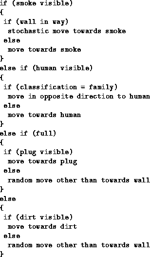
All strategies, hand-coded or learnt, must deal with the fact that there is no memory. Note that the hand-coded program implements a stochastic policy.
So why did Q-learning not find an optimal policy? The answer is because we are not using lookup tables, and we do not have time anyway to experience each full state. If the world was an MDP with lookup tables and we had infinite time, then yes, we couldn't beat ordinary Q-learning.
But because these conditions don't hold, we can go on and explore better action selection methods than Q-learning. Note that we don't actually know how good the optimum policy will be. As we shall see, we will be able to do a lot better than this, but will still not know at the end of the thesis if we have found the best possible solution.
Clearly, it is difficult to learn such a complex single mapping. We will now look at ways in which the learning problem may be broken up. First we test Hierarchical Q-learning.
To implement Hierarchical Q-learning in the House Robot problem,
we set the following 5 agents to build up personal ![]() values.
They learn by reference to personal reward functions
values.
They learn by reference to personal reward functions ![]() .
The switch then learns Q(x,i) from the global reward function as before.
.
The switch then learns Q(x,i) from the global reward function as before.
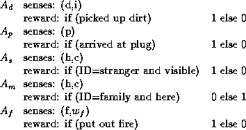
Each agent need only sense the subspace of ![]() that is relevant to its reward function.
To be precise, agent
that is relevant to its reward function.
To be precise, agent ![]() need only work with the minimum collection of senses
required to make
need only work with the minimum collection of senses
required to make
![]() ,
,
![]() stationary.[4]
There is no advantage to having the agents sense the full space for learning Q.
If it is given extra unnecessary senses, it will just learn
the same Q-values repeated.
stationary.[4]
There is no advantage to having the agents sense the full space for learning Q.
If it is given extra unnecessary senses, it will just learn
the same Q-values repeated.
For example, the plug-seeking agent ![]() has a reward function
has a reward function ![]() that only references the location of the plug,
so it need only sense (p).
Any extra senses will not affect the policy it learns
- it will suggest the same action independent of the values of
that only references the location of the plug,
so it need only sense (p).
Any extra senses will not affect the policy it learns
- it will suggest the same action independent of the values of ![]() .
It builds up
.
It builds up ![]() values where:
values where:
![]()
When the creature interacts with the world, each agent translates what is happening into its own subspace. For example (using the notation x,a -> y):

As well as requiring less memory, this builds up the Q-values much quicker. Here, all of the subspaces are small enough to use lookup tables.
The switch still sees the full state x,
and its Q(x,i) mapping needs to be implemented as a generalisation.
As before,
we reduce interference by breaking the state-action space up
into one network per "action" i.
The switch is implemented as 5 neural networks.
Each takes a vector input x and
produces a floating point output ![]() .
Each net is responsible for a different "action" i.
.
Each net is responsible for a different "action" i.
We try to keep the number of agents low, since a large number of agents will require a large (x,i) statespace. As before, we go through a number of trials, the switch replaying its experiences after each one.
Here the agents share the same suite of actions a = 0-8, but in general we may be interested in breaking up the action space also.
The agents can all learn their Q-values together in parallel.
The agent ![]() that suggested the executed action
that suggested the executed action ![]() can update:
can update:
![]()
If the agents share the same suite of actions (which we don't assume in general) then in fact all other agents can learn at same time. We can update for all i:
![]()
using their different reward functions ![]() .
We can do this because Q-learning is asynchronous and sampled
(we can learn from the single transition,
no matter what came before and no matter
what will come after).[5]
.
We can do this because Q-learning is asynchronous and sampled
(we can learn from the single transition,
no matter what came before and no matter
what will come after).[5]
We must ensure, when learning together, that all agents experience a large number of visits to each of their (x,a). An agent shouldn't miss out on some (x,a) just because other agents are winning. I simply use random winners during this collective Q-learning phase.
If an agent is of the form:
reward: if (good event) r else s
where r > s ,
then it is irrelevant what r and s actually are,
the agent will still learn the same policy (Theorem C.1).
So in particular setting r = 1 and s = 0 here
doesn't reduce our options.
If we replace 1 above by any number > 0 ,
the agent still learns the same pattern of behavior.
It still sends the same preferred action ![]() to the switch.
to the switch.
This does not hold for reward functions with
3 or more rewards,
where relative difference between rewards
will lead to different policies.
We mentioned that it can be difficult to write a reward function
so that maximising the rewards solves your problem.
For 3-reward (or more) reward functions
such as our global reward function,
experiment quickly shows that it is not simply a matter of
![]() for all good things
and
for all good things
and ![]() for all bad things.
for all bad things.
It can be difficult to predict what behavior maximising the rewards will lead to. For example, because it looks at future rewards, an agent may voluntarily suffer a punishment now in order to gain a high reward later, so simply coding a punishment for a certain transition may not be enough to ensure the agent avoids that transition. Reward functions are the "black art" of Reinforcement Learning, the place where design comes in. RL papers often list unintuitive and apparently arbitrary reward schemes which one realises may be the result of a lengthy process of trial-and-error.
To summarise, much attention has been given to breaking up the statespace of large problems, but the reward functions do not scale well either. Multi-reward functions like our global reward function are hard to design. It is much easier to design specialised 2- or 3-reward local functions (these 2-reward functions could not be easier to design: 1 for the good thing and 0 otherwise will do). Hierarchical Q-learning has not got rid of the global reward function, but we shall be attempting to do that later.
With the same replay strategy as before, and the same number of test runs, the Hierarchical Q-learning system scored 13.641 points per 100 steps, a considerable improvement on the single Q-learner. This is also considerably better than the hand-coded program - now we see that the optimum is not any strict hierarchy of goals. Rather some interleaving of goals is necessary.
Again though, Hierarchical Q-learning did not find an optimal policy.
We are going to introduce methods which will perform even better.
It did not find an optimal
![]() policy
because again, we are not using lookup tables,
and do not have time anyway to experience each full state.
policy
because again, we are not using lookup tables,
and do not have time anyway to experience each full state.
 per timestep.
Every 10 timesteps, an existing fire grows
by a random walk of 1 square.
[2] The same would hold if our input x was a vector of real numbers. In this case we could also use neural networks but they would be of a different architecture to the ones described here. Note also that in this case we effectively can't see the same state twice.
[3]
If we had a large action space, the actions would need to be generalised too,
e.g. we could have a single neural net with vector input x,a and a single floating point output Q(x,a).
The problem then is to calculate the  term
- we can't enumerate the actions.
See [Kaelbling et al., 1996,
§6.2] for a survey of generalising action spaces.
[4] That is, if the full-statespace transitions were stationary to begin with.
[5] Note that in [Humphrys, 1995, §3] I assumed that agents share the same suite of actions.
Return to Contents page.